鸢尾花的例子

监督学习问题：预测花的品种

数据分类：花瓣：长度，宽度；花萼：长度，宽度 单位厘米
花的品种：setosa，versicolor，virginica
目标：构建机器学习模型，从已有的测量数据进行学习，预测新花的品种

1.认识数据

加载必要的库

import numpy as np #矩阵运算
import matplotlib.pyplot as plt  #绘图
import pandas as pd  #基于numpy的数据分析库
import mglearn #美化图像

鸢尾花(iris)数据集，是机器学习和统计学中一个经典的数据集

包含在scikit-learn的datasets模块中

可以通过调用load_iris函数来加载数据

scikit是一个建立在Scipy基础上用于机器学习的python模块，包含众多顶级机器学习算法

Scipy包含的功能有最优化、线性代数、积分、插值、拟合、特殊函数、快速傅里叶变换、信号处理和图像处理、常微分方程求解和其他科学与工程中常用的计算
Scipy是一个用于数学、科学、工程领域的常用软件包，可以处理插值、积分、优化、图像处理、常微分方程数值解的求解、信号处理等问题。它用于有效计算Numpy矩阵，使Numpy和Scipy协同工作，高效解决问题。

from sklearn.datasets import load_iris
iris_dataset=load_iris()
print("keys of iris_dataset: \n{}".format(iris_dataset.keys()))

keys of iris_dataset: 
dict_keys(['data', 'target', 'target_names', 'DESCR', 'feature_names', 'filename'])

load_iris返回的iris对象是一个Bunch对象，包含键，值，以下输出各个键对应的数据

for i in iris_dataset.keys():
    print(str(i)+'对应值为：')
    print(iris_dataset[i],end='\n')
    

data对应值为：
[[5.1 3.5 1.4 0.2]
 [4.9 3.  1.4 0.2]
 [4.7 3.2 1.3 0.2]
 [4.6 3.1 1.5 0.2]
 [5.  3.6 1.4 0.2]
 [5.4 3.9 1.7 0.4]
 [4.6 3.4 1.4 0.3]
 [5.  3.4 1.5 0.2]
 [4.4 2.9 1.4 0.2]
 [4.9 3.1 1.5 0.1]
 [5.4 3.7 1.5 0.2]
 [4.8 3.4 1.6 0.2]
 [4.8 3.  1.4 0.1]
 [4.3 3.  1.1 0.1]
 [5.8 4.  1.2 0.2]
 [5.7 4.4 1.5 0.4]
 [5.4 3.9 1.3 0.4]
 [5.1 3.5 1.4 0.3]
 [5.7 3.8 1.7 0.3]
 [5.1 3.8 1.5 0.3]
 [5.4 3.4 1.7 0.2]
 [5.1 3.7 1.5 0.4]
 [4.6 3.6 1.  0.2]
 [5.1 3.3 1.7 0.5]
 [4.8 3.4 1.9 0.2]
 [5.  3.  1.6 0.2]
 [5.  3.4 1.6 0.4]
 [5.2 3.5 1.5 0.2]
 [5.2 3.4 1.4 0.2]
 [4.7 3.2 1.6 0.2]
 [4.8 3.1 1.6 0.2]
 [5.4 3.4 1.5 0.4]
 [5.2 4.1 1.5 0.1]
 [5.5 4.2 1.4 0.2]
 [4.9 3.1 1.5 0.2]
 [5.  3.2 1.2 0.2]
 [5.5 3.5 1.3 0.2]
 [4.9 3.6 1.4 0.1]
 [4.4 3.  1.3 0.2]
 [5.1 3.4 1.5 0.2]
 [5.  3.5 1.3 0.3]
 [4.5 2.3 1.3 0.3]
 [4.4 3.2 1.3 0.2]
 [5.  3.5 1.6 0.6]
 [5.1 3.8 1.9 0.4]
 [4.8 3.  1.4 0.3]
 [5.1 3.8 1.6 0.2]
 [4.6 3.2 1.4 0.2]
 [5.3 3.7 1.5 0.2]
 [5.  3.3 1.4 0.2]
 [7.  3.2 4.7 1.4]
 [6.4 3.2 4.5 1.5]
 [6.9 3.1 4.9 1.5]
 [5.5 2.3 4.  1.3]
 [6.5 2.8 4.6 1.5]
 [5.7 2.8 4.5 1.3]
 [6.3 3.3 4.7 1.6]
 [4.9 2.4 3.3 1. ]
 [6.6 2.9 4.6 1.3]
 [5.2 2.7 3.9 1.4]
 [5.  2.  3.5 1. ]
 [5.9 3.  4.2 1.5]
 [6.  2.2 4.  1. ]
 [6.1 2.9 4.7 1.4]
 [5.6 2.9 3.6 1.3]
 [6.7 3.1 4.4 1.4]
 [5.6 3.  4.5 1.5]
 [5.8 2.7 4.1 1. ]
 [6.2 2.2 4.5 1.5]
 [5.6 2.5 3.9 1.1]
 [5.9 3.2 4.8 1.8]
 [6.1 2.8 4.  1.3]
 [6.3 2.5 4.9 1.5]
 [6.1 2.8 4.7 1.2]
 [6.4 2.9 4.3 1.3]
 [6.6 3.  4.4 1.4]
 [6.8 2.8 4.8 1.4]
 [6.7 3.  5.  1.7]
 [6.  2.9 4.5 1.5]
 [5.7 2.6 3.5 1. ]
 [5.5 2.4 3.8 1.1]
 [5.5 2.4 3.7 1. ]
 [5.8 2.7 3.9 1.2]
 [6.  2.7 5.1 1.6]
 [5.4 3.  4.5 1.5]
 [6.  3.4 4.5 1.6]
 [6.7 3.1 4.7 1.5]
 [6.3 2.3 4.4 1.3]
 [5.6 3.  4.1 1.3]
 [5.5 2.5 4.  1.3]
 [5.5 2.6 4.4 1.2]
 [6.1 3.  4.6 1.4]
 [5.8 2.6 4.  1.2]
 [5.  2.3 3.3 1. ]
 [5.6 2.7 4.2 1.3]
 [5.7 3.  4.2 1.2]
 [5.7 2.9 4.2 1.3]
 [6.2 2.9 4.3 1.3]
 [5.1 2.5 3.  1.1]
 [5.7 2.8 4.1 1.3]
 [6.3 3.3 6.  2.5]
 [5.8 2.7 5.1 1.9]
 [7.1 3.  5.9 2.1]
 [6.3 2.9 5.6 1.8]
 [6.5 3.  5.8 2.2]
 [7.6 3.  6.6 2.1]
 [4.9 2.5 4.5 1.7]
 [7.3 2.9 6.3 1.8]
 [6.7 2.5 5.8 1.8]
 [7.2 3.6 6.1 2.5]
 [6.5 3.2 5.1 2. ]
 [6.4 2.7 5.3 1.9]
 [6.8 3.  5.5 2.1]
 [5.7 2.5 5.  2. ]
 [5.8 2.8 5.1 2.4]
 [6.4 3.2 5.3 2.3]
 [6.5 3.  5.5 1.8]
 [7.7 3.8 6.7 2.2]
 [7.7 2.6 6.9 2.3]
 [6.  2.2 5.  1.5]
 [6.9 3.2 5.7 2.3]
 [5.6 2.8 4.9 2. ]
 [7.7 2.8 6.7 2. ]
 [6.3 2.7 4.9 1.8]
 [6.7 3.3 5.7 2.1]
 [7.2 3.2 6.  1.8]
 [6.2 2.8 4.8 1.8]
 [6.1 3.  4.9 1.8]
 [6.4 2.8 5.6 2.1]
 [7.2 3.  5.8 1.6]
 [7.4 2.8 6.1 1.9]
 [7.9 3.8 6.4 2. ]
 [6.4 2.8 5.6 2.2]
 [6.3 2.8 5.1 1.5]
 [6.1 2.6 5.6 1.4]
 [7.7 3.  6.1 2.3]
 [6.3 3.4 5.6 2.4]
 [6.4 3.1 5.5 1.8]
 [6.  3.  4.8 1.8]
 [6.9 3.1 5.4 2.1]
 [6.7 3.1 5.6 2.4]
 [6.9 3.1 5.1 2.3]
 [5.8 2.7 5.1 1.9]
 [6.8 3.2 5.9 2.3]
 [6.7 3.3 5.7 2.5]
 [6.7 3.  5.2 2.3]
 [6.3 2.5 5.  1.9]
 [6.5 3.  5.2 2. ]
 [6.2 3.4 5.4 2.3]
 [5.9 3.  5.1 1.8]]
target对应值为：
[0 0 0 0 0 0 0 0 0 0 0 0 0 0 0 0 0 0 0 0 0 0 0 0 0 0 0 0 0 0 0 0 0 0 0 0 0
 0 0 0 0 0 0 0 0 0 0 0 0 0 1 1 1 1 1 1 1 1 1 1 1 1 1 1 1 1 1 1 1 1 1 1 1 1
 1 1 1 1 1 1 1 1 1 1 1 1 1 1 1 1 1 1 1 1 1 1 1 1 1 1 2 2 2 2 2 2 2 2 2 2 2
 2 2 2 2 2 2 2 2 2 2 2 2 2 2 2 2 2 2 2 2 2 2 2 2 2 2 2 2 2 2 2 2 2 2 2 2 2
 2 2]
target_names对应值为：
['setosa' 'versicolor' 'virginica']
DESCR对应值为：
.. _iris_dataset:

Iris plants dataset
--------------------

**Data Set Characteristics:**

    :Number of Instances: 150 (50 in each of three classes)
    :Number of Attributes: 4 numeric, predictive attributes and the class
    :Attribute Information:
        - sepal length in cm
        - sepal width in cm
        - petal length in cm
        - petal width in cm
        - class:
                - Iris-Setosa
                - Iris-Versicolour
                - Iris-Virginica
                
    :Summary Statistics:

    ============== ==== ==== ======= ===== ====================
                    Min  Max   Mean    SD   Class Correlation
    ============== ==== ==== ======= ===== ====================
    sepal length:   4.3  7.9   5.84   0.83    0.7826
    sepal width:    2.0  4.4   3.05   0.43   -0.4194
    petal length:   1.0  6.9   3.76   1.76    0.9490  (high!)
    petal width:    0.1  2.5   1.20   0.76    0.9565  (high!)
    ============== ==== ==== ======= ===== ====================

    :Missing Attribute Values: None
    :Class Distribution: 33.3% for each of 3 classes.
    :Creator: R.A. Fisher
    :Donor: Michael Marshall (MARSHALL%PLU@io.arc.nasa.gov)
    :Date: July, 1988

The famous Iris database, first used by Sir R.A. Fisher. The dataset is taken
from Fisher's paper. Note that it's the same as in R, but not as in the UCI
Machine Learning Repository, which has two wrong data points.

This is perhaps the best known database to be found in the
pattern recognition literature.  Fisher's paper is a classic in the field and
is referenced frequently to this day.  (See Duda & Hart, for example.)  The
data set contains 3 classes of 50 instances each, where each class refers to a
type of iris plant.  One class is linearly separable from the other 2; the
latter are NOT linearly separable from each other.

.. topic:: References

   - Fisher, R.A. "The use of multiple measurements in taxonomic problems"
     Annual Eugenics, 7, Part II, 179-188 (1936); also in "Contributions to
     Mathematical Statistics" (John Wiley, NY, 1950).
   - Duda, R.O., & Hart, P.E. (1973) Pattern Classification and Scene Analysis.
     (Q327.D83) John Wiley & Sons.  ISBN 0-471-22361-1.  See page 218.
   - Dasarathy, B.V. (1980) "Nosing Around the Neighborhood: A New System
     Structure and Classification Rule for Recognition in Partially Exposed
     Environments".  IEEE Transactions on Pattern Analysis and Machine
     Intelligence, Vol. PAMI-2, No. 1, 67-71.
   - Gates, G.W. (1972) "The Reduced Nearest Neighbor Rule".  IEEE Transactions
     on Information Theory, May 1972, 431-433.
   - See also: 1988 MLC Proceedings, 54-64.  Cheeseman et al"s AUTOCLASS II
     conceptual clustering system finds 3 classes in the data.
   - Many, many more ...
feature_names对应值为：
['sepal length (cm)', 'sepal width (cm)', 'petal length (cm)', 'petal width (cm)']
filename对应值为：
E:\Python\Anaconda\lib\site-packages\sklearn\datasets\data\iris.csv

对数据进行说明：
data：每一行4个数对应花瓣的长宽，花萼的长宽

target：每一朵花对应的类别，0,1,2对应target_name的下标

target_name:花的类别集合

DESCR：数据集的简要说明

feature_name：数据说明，声明每一个特征

(机器学习中的个体叫做样本，其属性叫做特征)

2.训练和测试数据

构建机器学习模型

已有数据集分为两部分，一部分构建模型，一部分测试模型

scikit-learn中的train_test_split函数可以打乱数据集并进行拆分

将75%的行数据及对应标签作为训练集，25%作为训练集，这是推荐分配方式

scikit-learn 中的数据通常用大写的 X 表示，而标签用小写的 y 表示。

这是受到了数学标准公式 f(x)=y 的启发，其中 x 是函数的输入，y 是输出。我们用大写的 X 是因为数据是一个二维数组（矩阵），用小写的 y 是因为目标是一个一维数组（向量），这也是数学中的约定。

对数据调用train_test_split划分数据集

from sklearn.model_selection import train_test_split
X_train,X_test,y_train,y_test=train_test_split(iris_dataset['data'],
iris_dataset['target'],random_state=0) #为了保证多次运行同一函数能得到相同输出，利用random_state指定了生成随机参数的种子
#输出的结果都是Numpy数组

print("X_train shape: {}".format(X_train.shape))
print("y_train shape: {}".format(y_train.shape))

X_train shape: (112, 4)
y_train shape: (112,)

print("x_test shape: {}".format(X_test.shape))
print("y_test shape: {}".format(y_test.shape))

x_test shape: (38, 4)
y_test shape: (38,)

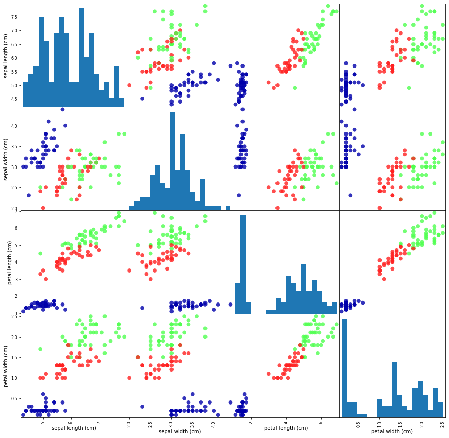
3.观察数据

构建机器学习模型之前，检测数据，排查异常数据

利用数据可视化：

• 绘制散点图：分为x，y轴，一次只能绘制两个特征
• 绘制散点图矩阵：无法同时显示所有特征之间的关系

利用pandas的scatter_matrix函数绘制散点图矩阵

参数解释:

frame：数据的dataframe,本例为4150的矩阵;

c是颜色,本例中按照y_train的不同来分配不同的颜色;

figsize设置图片的尺寸;

marker是散点的形状,’o’是圆形,’‘是星形 ;

hist_kwds是直方图的相关参数,{‘bins’:20}是生成包含20个长条的直方图;

s是大图的尺寸 ;

alpha是图的透明度;

cmap是colourmap,就是颜色板

import pandas as pd
import mglearn
#利用X_train中的数据创建DataFrame
#利用iris_dataset.feature_names中的字符串对数据列进行标记
iris_dataframe=pd.DataFrame(X_train,columns=iris_dataset.feature_names)
#利用DataFrame创建散点图矩阵，按y_train着色
grr=pd.plotting.scatter_matrix(iris_dataframe,c=y_train,figsize=(15,15),marker='o',
                              hist_kwds={'bins':20},s=60,alpha=.8,cmap=mglearn.cm3)

4.KNN算法

开始构建机器学习模型

skikit-learn中有许多
可用的分类算法

这里采用k近邻算法：
考虑训练集中与新数据点最近的任意 k 个邻居（比如说，距离最近的 3 个或 5 个邻居），而不是只考虑最近的那一个。然后，我们可以用这些邻居中数量最多的类别做出预测

scikit-learn 中所有的机器学习模型都在各自的类中实现，这些类被称为 Estimator类。k 近邻分类算法是在 neighbors 模块的 KNeighborsClassifier 类中实现的。我们需要将这个类实例化为一个对象，然后才能使用这个模型。这时我们需要设置模型的参数。KNeighborsClassifier 最重要的参数就是邻居的数目，这里我们设为 1 ：

from sklearn.neighbors import KNeighborsClassifier
knn=KNeighborsClassifier(n_neighbors=1)

想要基于训练集来构建模型，需要调用 knn 对象的 fit 方法，输入参数为 X_train 和 y_train

二者都是 NumPy 数组，前者包含训练数据，后者包含相应的训练标签

knn.fit(X_train,y_train)

KNeighborsClassifier(algorithm='auto', leaf_size=30, metric='minkowski',
                     metric_params=None, n_jobs=None, n_neighbors=1, p=2,
                     weights='uniform')

5.预测和评估

y_pred=knn.predict(X_test)
print("Test set predictions:\n {}".format(y_pred))

Test set predictions:
 [2 1 0 2 0 2 0 1 1 1 2 1 1 1 1 0 1 1 0 0 2 1 0 0 2 0 0 1 1 0 2 1 0 2 2 1 0
 2]

print("Test set score: {:.2f}".format(np.mean(y_pred==y_test)))

Test set score: 0.97

对于这个模型来说，测试集的精度约为 0.97，也就是说，对于测试集中的鸢尾花，我们的预测有 97% 是正确的。根据一些数学假设，对于新的鸢尾花，可以认为我们的模型预测结果有 97% 都是正确的。

完整代码如下：

import numpy as np #矩阵运算
import matplotlib.pyplot as plt  #绘图
import pandas as pd  #基于numpy的数据分析库
import mglearn #美化图像
from sklearn.model_selection import train_test_split
from sklearn.neighbors import KNeighborsClassifier
iris_dataset=load_iris()
X_train,X_test,y_train,y_test=train_test_split(iris_dataset['data'],
iris_dataset['target'],random_state=0) #为了保证多次运行同一函数能得到相同输出，利用random_state指定了生成随机参数的种子
#输出的结果都是Numpy数组
#利用X_train中的数据创建DataFrame
#利用iris_dataset.feature_names中的字符串对数据列进行标记
iris_dataframe=pd.DataFrame(X_train,columns=iris_dataset.feature_names)
#利用DataFrame创建散点图矩阵，按y_train着色
grr=pd.plotting.scatter_matrix(iris_dataframe,c=y_train,figsize=(15,15),marker='o',
                              hist_kwds={'bins':20},s=60,alpha=.8,cmap=mglearn.cm3)
knn=KNeighborsClassifier(n_neighbors=1)
knn.fit(X_train,y_train)
y_pred=knn.predict(X_test)
print("Test set score: {:.2f}".format(np.mean(y_pred==y_test)))

Test set score: 0.97