监督学习之k近邻 所需要的所有包 1 2 3 4 5 6 7 8 import numpy as npimport matplotlib.pyplot as pltimport pandas as pdimport mglearn
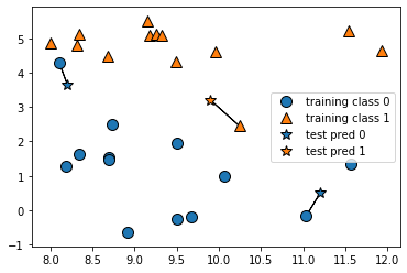
1.k近邻分类 1 2 3 4 import mglearn1 )
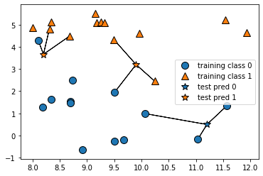
除了仅考虑最近邻,我还可以考虑任意个(k 个)邻居。这也是 k 近邻算法名字的来历。在考虑多于一个邻居的情况时,我们用“投票法”(voting)来指定标签 。也就是说,对于每个测试点,我们数一数多少个邻居属于类别 0,多少个邻居属于类别 1。然后将出现次数更多的类别(也就是 k 个近邻中占多数的类别)作为预测结果 。下面的例子(图 2-5)用到了 3 个近邻:
1 mglearn.plots.plot_knn_classification(n_neighbors=3 )
通过scikit-learn来应用k近邻算法
导入类并将其实例化。这时可以设定参数,如邻居的个数
利用训练集对这个分类器进行拟合
调用 predict 方法来对测试数据进行预测
1 2 3 4 5 6 7 8 9 from sklearn.model_selection import train_test_split0 )from sklearn.neighbors import KNeighborsClassifier3 )print ("Test set predictions: {}" .format (clf.predict(X_test)))print ("Test set accuracy: {:.2f}" .format (clf.score(X_test,y_test)))
Test set predictions: [1 0 1 0 1 0 0]
Test set accuracy: 0.86
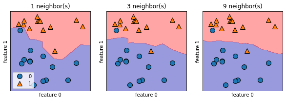
2.分析KNeighborsClassifier 对于二维数据集,我们还可以在 xy 平面上画出所有可能的测试点的预测结果。我们根据平面中每个点所属的类别对平面进行着色。这样可以查看决策边界(decision boundary),即算法对类别 0 和类别 1 的分界线。
zip() 函数用于将可迭代的对象作为参数,将对象中对应的元素打包成一个个元组,然后返回由这些元组组成的列表。
subplots参数与subplots相似。
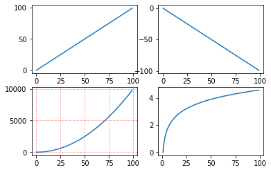
1 2 3 4 5 6 7 8 9 10 11 12 13 14 15 16 17 18 19 20 21 import numpy as npimport matplotlib.pyplot as plt0 , 100 )2 ,2 )0 ,0 ]0 ,1 ]1 ,0 ]1 ,1 ]2 )'r' , linestyle='--' , linewidth=1 ,alpha=0.3 )
1 2 3 4 5 6 7 8 9 fig,axes=plt.subplots(1 ,3 ,figsize=(10 ,3 ))for n_neighbors,ax in zip ([1 ,3 ,9 ],axes):True ,eps=0.5 ,ax=ax,alpha=.4 )0 ],X[:,1 ],y,ax=ax)"{} neighbor(s)" .format (n_neighbors))"feature 0" )"feature 1" )0 ].legend(loc=3 )
<matplotlib.legend.Legend at 0x242302ba9b0>
用单一邻居绘制的决策边界紧跟着训练数据。随着邻居个数越来越多,决策边界也越来越平滑。更平滑的边界对应更简单的模型。换句话说,使用更少的邻居对应更高的模型复杂度,而使用更多的邻居对应更低的模型复杂度。假如考虑极端情况,即邻居个数等于训练集中所有数据点的个数,那么每个测试点的邻居都完全相同(即所有训练点),所有预测结果也完全相同(即训练集中出现次数最多的类别)。
在现实世界的乳腺癌数据集上进行研究,证实模型复杂度和泛化能力的关系
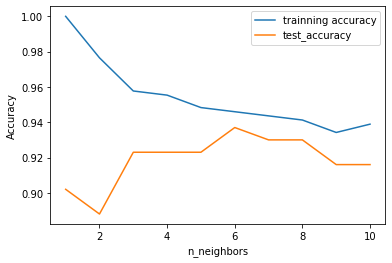
1 2 3 4 5 6 7 8 9 10 11 12 13 14 15 16 17 18 19 20 21 22 23 24 25 from sklearn.datasets import load_breast_cancerfrom sklearn.model_selection import train_test_splitfrom sklearn import neighbors66 )range (1 ,11 )for n_neighbors in neighbors_settings:"trainning accuracy" )"test_accuracy" )"Accuracy" )"n_neighbors" )
<matplotlib.legend.Legend at 0x24230a4b5c0>
仅考虑单一近邻时,训练集上的预测结果十分完美。但随着邻居个数的增多,模型变得更简单,训练集精度也随之下降。单一邻居时的测试集精度比使用更多邻居时要低,这表示单一近邻的模型过于复杂。与之相反,当考虑 10 个邻居时,模型又过于简单,性能甚至变得更差。最佳性能在中间的某处,邻居个数大约为 6。不过最好记住这张图的坐标轴刻度。最差的性能约为 88% 的精度,这个结果仍然可以接受。
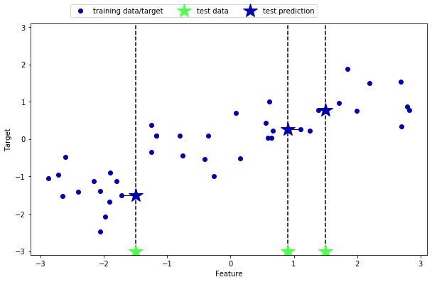
3.K近邻回归 k近邻算法还可以用于回归(把邻居的平均值赋给目标)。
1 mglearn.plots.plot_knn_regression(n_neighbors=1 )
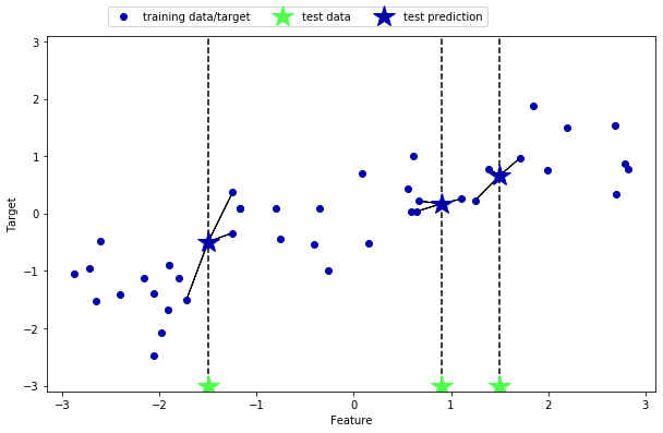
用多个近邻进行回归,预测结果为这些邻居的平均值
1 mglearn.plots.plot_knn_regression(n_neighbors=3 )
用于回归的k近邻算法在sklearn的KNeighborsRegressor类中实现
1 2 3 4 5 6 7 8 9 10 from sklearn.neighbors import KNeighborsRegressor40 )0 )3 )
KNeighborsRegressor(algorithm='auto', leaf_size=30, metric='minkowski',
metric_params=None, n_jobs=None, n_neighbors=3, p=2,
weights='uniform')
1 2 3 4 5 print ("Test set predictions:\n{}" .format (reg.predict(X_test)))print ("Test set R^2:{:.2f}" .format (reg.score(X_test,y_test)))
Test set predictions:
[-0.05396539 0.35686046 1.13671923 -1.89415682 -1.13881398 -1.63113382
0.35686046 0.91241374 -0.44680446 -1.13881398]
Test set R^2:0.83
可以用score方法来评估模型,对于回归问题,这一方法返回的是$R^2$分数,也叫做决定系数,是回归模型预测的优度度量,位于0到1之间,1完美预测,0对于常数模型,即总是预测训练集响应(y_train)的平均值
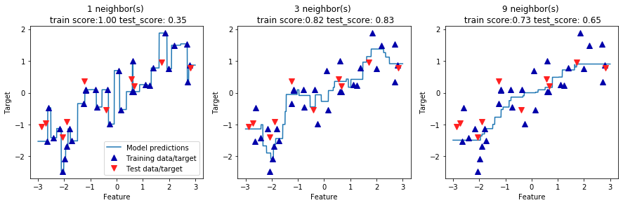
4.分析KNeigborsRegressor 对于我们的一维数据集,可以查看所有特征取值对应的预测结果(图 2-10)。为了便于绘
np reshape array linespace 用法:
1 2 3 import numpy as npprint (np.array([1 ,1 ,1 ]).reshape(3 ,1 ))
[[1]
[1]
[1]]
1 print (np.linspace(1 ,100 ,2 ).reshape(2 ,-1 ))
[[ 1.]
[100.]]
1 2 3 4 5 6 7 8 9 10 11 12 13 14 15 16 17 fig,axes=plt.subplots(1 ,3 ,figsize=(15 ,4 ))3 ,3 ,1000 ).reshape(-1 ,1 )for n_neighbors,ax in zip ([1 ,3 ,9 ],axes):'^' ,c=mglearn.cm2(0 ),markersize=8 )'v' ,c=mglearn.cm2(1 ),markersize=8 )"{} neighbor(s) \n train score:{:.2f} test_score: {:.2f}" .format ("Feature" )"Target" )0 ].legend(["Model predictions" ,"Training data/target" ,"Test data/target" ],loc="best" )
<matplotlib.legend.Legend at 0x2422e47e5c0>
从图中可以看出,仅使用单一邻居,训练集中的每个点都对预测结果有显著影响,预测结果的图像经过所有数据点。这导致预测结果非常不稳定。考虑更多的邻居之后,预测结果变得更加平滑,但对训练数据的拟合也不好。
5.优点,缺点和参数 一般来说, KNeighbors 分类器有 2 个重要参数:邻居个数与数据点之间距离的度量方法。在实践中,使用较小的邻居个数(比如 3 个或 5 个)往往可以得到比较好的结果,但你应该调节这个参数。选择合适的距离度量方法超出了本书的范围。默认使用欧式距离,它在许多情况下的效果都很好。
k-NN 的优点之一就是模型很容易理解,通常不需要过多调节就可以得到不错的性能。在考虑使用更高级的技术之前,尝试此算法是一种很好的基准方法。构建最近邻模型的速度通常很快,但如果训练集很大(特征数很多或者样本数很大),预测速度可能会比较慢。使用 k-NN 算法时,对数据进行预处理是很重要的(见第 3 章)。这一算法对于有很多特征(几百或更多)的数据集往往效果不好,对于大多数特征的大多数取值都为 0 的数据集(所谓的稀疏数据集)来说,这一算法的效果尤其不好。
虽然 k 近邻算法很容易理解,但由于预测速度慢且不能处理具有很多特征的数据集,所以在实践中往往不会用到