监督学习之线性模型

监督学习之线性模型

基本概念：

回归：统计学中，回归分析（regression analysis)指的是确定两种或两种以上变量间相互依赖的定量关系的一种统计分析方法。回归分析按照涉及的变量的多少，分为一元回归和多元回归分析；按照因变量的多少，可分为简单回归分析和多重回归分析；按照自变量和因变量之间的关系类型，可分为线性回归分析和非线性回归分析。

线性回归：

线性回归是利用数理统计中回归分析，来确定两种或两种以上变量间相互依赖的定量关系的一种统计分析方法，运用十分广泛。其表达形式为y = w’x+e，e为误差服从均值为0的正态分布。

回归分析中，只包括一个自变量和一个因变量，且二者的关系可用一条直线近似表示，这种回归分析称为一元线性回归分析。如果回归分析中包括两个或两个以上的自变量，且因变量和自变量之间是线性关系，则称为多元线性回归分析。

python中shape简易用法：

通过安装导入numpy库，矩阵（ndarray）的shape属性可以获取矩阵的形状（例如二维数组的行列），获取的结果是一个元组

shape[0] 行

shape[1] 列

import numpy as np
import pandas as pd
import matplotlib.pyplot as plt
import mglearn
%matplotlib inline

线性模型利用输入特征的线性函数进行预测

1.用于回归的线性模型

对于回归问题，线性模型预测的一般公式如下：

ŷ=w[0]∗x[0]+w[1]∗x[1]+…+w[p]∗x[p]+b

这里 x[0]
到 x[p] 表示单个数据点的特征（本例中特征个数为 p+1），w 和 b 是学习模型的
参数，ŷ

是模型的预测结果。对于单一特征的数据集，公式如下：

ŷ=w[0]∗x[0]+b

你可能还记得，这就是高中数学里的直线方程。这里 w[0]
是斜率，b 是 y 轴偏移。对于有
更多特征的数据集，w 包含沿每个特征坐标轴的斜率。或者，你也可以将预测的响应值看
作输入特征的加权求和，权重由 w 的元素给出（可以取负值）。
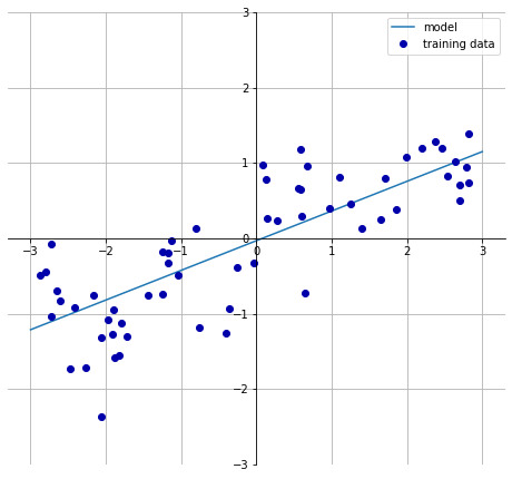
下列代码可以在一维 wave 数据集上学习参数 w[0] 和 b：

mglearn.plots.plot_linear_regression_wave()

w[0]: 0.393906  b: -0.031804

有许多不同的线性回归模型。

这些模型之间的区别在于如何从训练数据中学习参数 w 和 b，以及如何控制模型复杂度。

下面介绍最常见的线性回归模型。

2.线性回归

线性回归，或者普通最小二乘法（ordinary least squares，OLS），是回归问题最简单也最经典的线性方法。

线性回归寻找参数 w 和 b，使得对训练集的预测值与真实的回归目标值 y 之间的均方误差最小。

均方误差（mean squared error）是预测值与真实值之差的平方和除以样本数。

线性回归没有参数，这是一个优点，但也因此无法控制模型的复杂度。

from sklearn.linear_model import LinearRegression
from sklearn.model_selection import train_test_split
X,y=mglearn.datasets.make_wave(n_samples=60)
X_train,X_test,y_train,y_test=train_test_split(X,y,random_state=42)
lr=LinearRegression().fit(X_train,y_train)

“斜率”参数（w，也叫作权重或系数）被保存在 coef_ 属性中，而偏移或截距（b）被保存在 intercept_ 属性中：

print("lr.coef_:{}".format(lr.coef_))
print("lr.intercept_:{}".format(lr.intercept_))

lr.coef_:[0.39390555]
lr.intercept_:-0.031804343026759746

你可能注意到了 coef_ 和 intercept_ 结尾处奇怪的下划线。scikit-learn 总是将从训练数据中得出的值保存在以下划线结尾的属性中。这是为了将其与用户设置的参数区分开。

intercept_ 属性是一个浮点数，而 coef_ 属性是一个 NumPy 数组，每个元素对应一个输入特征。由于 wave 数据集中只有一个输入特征，所以 lr.coef_ 中只有一个元素。我们来看一下训练集和测试集的性能：

print("Training set score: {:.2f}".format(lr.score(X_train, y_train)))
print("Test set score: {:.2f}".format(lr.score(X_test, y_test)))

Training set score: 0.67
Test set score: 0.66

对于更高维的数据集（即有大量特征的数据集），线性模型将变得更加强大，过拟合的可能性也会变大。我们来看一下 LinearRegression 在更复杂的数据集上的表现，比如波士顿房价数据集。记住，这个数据集有 506 个样本和 105个导出特征。首先，加载数据集并将其分为训练集和测试集。然后像前面一样构建线性回归模型：

X,y=mglearn.datasets.load_extended_boston()
X_train,X_test,y_train,y_test=train_test_split(X,y,random_state=0)
lr=LinearRegression().fit(X_train, y_train)
print("Trainnig set score: {:.2f}".format(lr.score(X_train,y_train)))
print("Test set score: {:.2f}".format(lr.score(X_test,y_test)))

Trainnig set score: 0.95
Test set score: 0.61

训练集和测试集之间的性能差异是过拟合的明显标志，因此我们应该试图找到一个可以控制复杂度的模型。标准线性回归最常用的替代方法之一就是岭回归（ridge regression），下面来看一下。


过拟合：一个假设在训练数据上能够获得比其他假设更好的拟合， 但是在训练数据外的数据集上却不能很好地拟合数据，此时认为这个假设出现了过拟合的现象。出现这种现象的主要原因是训练数据中存在噪音或者训练数据太少。

3.岭回归

岭回归也是一种用于回归的线性模型，因此它的预测公式与普通最小二乘法相同。但在岭回归中，对系数（w）的选择不仅要在训练数据上得到好的预测结果，而且还要拟合附加约束。我们还希望系数尽量小。换句话说，w 的所有元素都应接近于 0。直观上来看，这意味着每个特征对输出的影响应尽可能小（即斜率很小），同时仍给出很好的预测结果。这种约束是所谓正则化（regularization）的一个例子。正则化是指对模型做显式约束，以避免过拟合。岭回归用到的这种被称为 L2 正则化。

岭回归在 linear_model.Ridge 中实现。来看一下它对扩展的波士顿房价数据集的效果如何

from sklearn.linear_model import Ridge
ridge=Ridge().fit(X_train,y_train)
print("Training set score: {:.2f}".format(ridge.score(X_train, y_train)))
print("Test set score: {:.2f}".format(ridge.score(X_test, y_test)))

Training set score: 0.89
Test set score: 0.75

可以看出， Ridge 在训练集上的分数要低于 LinearRegression ，但在测试集上的分数更高。这和我们的预期一致。线性回归对数据存在过拟合。 Ridge 是一种约束更强的模型，所以更不容易过拟合。复杂度更小的模型意味着在训练集上的性能更差，但泛化性能更好。由于我们只对泛化性能感兴趣，所以应该选择 Ridge 模型而不是 LinearRegression 模型。

Ridge 模型在模型的简单性（系数都接近于 0）与训练集性能之间做出权衡。简单性和训练集性能二者对于模型的重要程度可以由用户通过设置 alpha 参数来指定。在前面的例子中，我们用的是默认参数 alpha=1.0 。但没有理由认为这会给出最佳权衡。 alpha 的最佳设定值取决于用到的具体数据集。增大 alpha 会使得系数更加趋向于 0，从而降低训练集性能，但可能会提高泛化性能。例如：

ridge10=Ridge(alpha=10).fit(X_train,y_train)
print("Training set score: {:.2f}".format(ridge10.score(X_train, y_train)))
print("Test set score: {:.2f}".format(ridge10.score(X_test, y_test)))

Training set score: 0.79
Test set score: 0.64

减小 alpha 可以让系数受到的限制更小。对于非常小的 alpha 值，系数几乎没有受到限制，我们得到一个与 LinearRegression 类似的模型：

ridge01=Ridge(alpha=0.1).fit(X_train,y_train)
print("Training set score: {:.2f}".format(ridge01.score(X_train, y_train)))
print("Test set score: {:.2f}".format(ridge01.score(X_test, y_test)))

Training set score: 0.93
Test set score: 0.77

这里 alpha=0.1 似乎效果不错。我们可以尝试进一步减小 alpha 以提高泛化性能。

我们还可以查看 alpha 取不同值时模型的 coef_ 属性，从而更加定性地理解 alpha 参数是如何改变模型的。更大的 alpha 表示约束更强的模型，所以我们预计大 alpha 对应的 coef_ 元素比小 alpha 对应的 coef_ 元素要小。

plt.plot(ridge.coef_, 's', label="Ridge alpha=1")
plt.plot(ridge10.coef_, '^', label="Ridge alpha=10")
plt.plot(ridge01.coef_, 'v', label="Ridge alpha=0.1")
plt.plot(lr.coef_, 'o', label="LinearRegression")
plt.xlabel("Coefficient index")
plt.ylabel("Coefficient magnitude")
plt.hlines(0, 0, len(lr.coef_))
plt.ylim(-25, 25)
plt.legend()

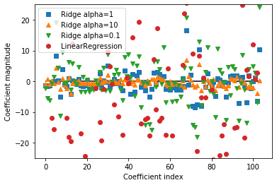
这里 x 轴对应 coef_ 的元素： x=0 对应第一个特征的系数， x=1 对应第二个特征的系数，以此类推，一直到 x=100 。y 轴表示该系数的具体数值。这里需要记住的是，对于 alpha=10 ，系数大多在 -3 和 3 之间。对于 alpha=1 的 Ridge 模型，系数要稍大一点。对于 alpha=0.1 ，点的范围更大。对于没有做正则化的线性回归（即 alpha=0 ），点的范围很大，许多点都超出了图像的范围。

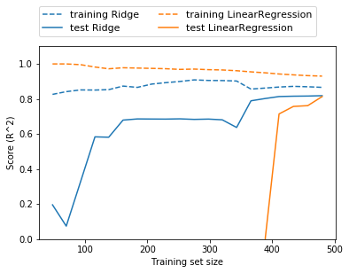
还有一种方法可以用来理解正则化的影响，就是固定 alpha 值，但改变训练数据量。我们对波士顿房价数据集做二次抽样，并在数据量逐渐增加的子数据集上分别对 LinearRegression 和 Ridge(alpha=1) 两个模型进行评估（将模型性能作为数据集大小的函数进行绘图，这样的图像叫作学习曲线):

mglearn.plots.plot_ridge_n_samples()

4.lasso

除了 Ridge ，还有一种正则化的线性回归是 Lasso 。与岭回归相同，使用 lasso 也是约束系数使其接近于 0，但用到的方法不同，叫作 L1 正则化。L1 正则化的结果是，使用 lasso 时某些系数刚好为 0。这说明某些特征被模型完全忽略。这可以看作是一种自动化的特征选择。某些系数刚好为 0，这样模型更容易解释，也可以呈现模型最重要的特征。

我们将 lasso 应用在扩展的波士顿房价数据集上：

from sklearn.linear_model import Lasso
lasso=Lasso().fit(X_train,y_train)
print("Training set score: {:.2f}".format(lasso.score(X_train, y_train)))
print("Test set score: {:.2f}".format(lasso.score(X_test, y_test)))
print("Number of features used: {}".format(np.sum(lasso.coef_ != 0)))
print("Number of all feature: {}".format(lasso.coef_.shape[0]))

Training set score: 0.29
Test set score: 0.21
Number of features used: 4
Number of all feature: 104

如你所见， Lasso 在训练集与测试集上的表现都很差。这表示存在欠拟合，我们发现模型只用到了 105 个特征中的 4 个。与 Ridge 类似， Lasso 也有一个正则化参数 alpha ，可以控制系数趋向于 0 的强度。在上一个例子中，我们用的是默认值 alpha=1.0 。为了降低欠拟合，我们尝试减小 alpha 。这么做的同时，我们还需要增加 max_iter 的值（运行迭代的最大次数）：

# 我们增大max_iter的值，否则模型会警告我们，说应该增大max_iter
lasso001 = Lasso(alpha=0.01, max_iter=100000).fit(X_train, y_train)
print("Training set score: {:.2f}".format(lasso001.score(X_train, y_train)))
print("Test set score: {:.2f}".format(lasso001.score(X_test, y_test)))
print("Number of features used: {}".format(np.sum(lasso001.coef_ != 0)))

Training set score: 0.90
Test set score: 0.77
Number of features used: 33

alpha 值变小，我们可以拟合一个更复杂的模型，在训练集和测试集上的表现也更好。模型性能比使用 Ridge 时略好一点，而且我们只用到了 105 个特征中的 33 个。这样模型可能更容易理解。

但如果把 alpha 设得太小，那么就会消除正则化的效果，并出现过拟合，得到与LinearRegression 类似的结果：

lasso00001 = Lasso(alpha=0.0001, max_iter=100000).fit(X_train, y_train)
print("Training set score: {:.2f}".format(lasso00001.score(X_train, y_train)))
print("Test set score: {:.2f}".format(lasso00001.score(X_test, y_test)))
print("Number of features used: {}".format(np.sum(lasso00001.coef_ != 0)))

Training set score: 0.95
Test set score: 0.64
Number of features used: 96

对不同模型的系数进行作图

plt.plot(lasso.coef_, 's', label="Lasso alpha=1")
plt.plot(lasso001.coef_, '^', label="Lasso alpha=0.01")
plt.plot(lasso00001.coef_, 'v', label="Lasso alpha=0.0001")
plt.plot(ridge01.coef_, 'o', label="Ridge alpha=0.1")
plt.legend(ncol=2, loc=(0, 1.05))
plt.ylim(-25, 25)
plt.xlabel("Coefficient index")
plt.ylabel("Coefficient magnitude")

Text(0, 0.5, 'Coefficient magnitude')

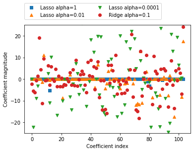
在 alpha=1 时，我们发现不仅大部分系数都是 0（我们已经知道这一点），而且其他系数也都很小。将 alpha 减小至 0.01 ，我们得到图中向上的三角形，大部分特征等于 0。alpha=0.0001 时，我们得到正则化很弱的模型，大部分系数都不为 0，并且还很大。为了便于比较，图中用圆形表示 Ridge 的最佳结果。 alpha=0.1 的 Ridge 模型的预测性能与alpha=0.01 的 Lasso 模型类似，但 Ridge 模型的所有系数都不为 0。

在实践中，在两个模型中一般首选岭回归。但如果特征很多，你认为只有其中几个是重要的，那么选择 Lasso 可能更好。同样，如果你想要一个容易解释的模型， Lasso 可以给出更容易理解的模型，因为它只选择了一部分输入特征。 scikit-learn 还提供了 ElasticNet类，结合了 Lasso 和 Ridge 的惩罚项。在实践中，这种结合的效果最好，不过代价是要调节两个参数：一个用于 L1 正则化，一个用于 L2 正则化。

5.用于分类的线性模型

线性模型也广泛应用于分类问题。我们首先来看二分类。这时可以利用下面的公式进行
预测：

ŷ =w[0]∗x[0]+w[1]∗x[1]+…+w[p]∗x[p]+b>0

这个公式看起来与线性回归的公式非常相似，但我们没有返回特征的加权求和，而是为预测设置了阈值（0）。如果函数值小于 0，我们就预测类别 -1；如果函数值大于 0，我们就预测类别 +1。对于所有用于分类的线性模型，这个预测规则都是通用的。同样，有很多种不同的方法来找出系数（w）和截距（b）。

对于用于回归的线性模型，输出 ŷ 是特征的线性函数，是直线、平面或超平面（对于更高维的数据集）。对于用于分类的线性模型，决策边界是输入的线性函数。换句话说，（二元）线性分类器是利用直线、平面或超平面来分开两个类别的分类器。本节我们将看到这方面的例子。

学习线性模型有很多种算法。这些算法的区别在于以下两点：

系数和截距的特定组合对训练数据拟合好坏的度量方法；
是否使用正则化，以及使用哪种正则化方法。

不同的算法使用不同的方法来度量“对训练集拟合好坏”。由于数学上的技术原因，不可能调节 w 和 b 使得算法产生的误分类数量最少。对于我们的目的，以及对于许多应用而言，上面第一点（称为损失函数）的选择并不重要。

最常见的两种线性分类算法是 Logistic 回归（logistic regression）和线性支持向量机（linear support vector machine，线性 SVM），前者在 linear_model.LogisticRegression 中实现，后者在 svm.LinearSVC （SVC 代表支持向量分类器）中实现。虽然 LogisticRegression的名字中含有回归（regression），但它是一种分类算法，并不是回归算法，不应与LinearRegression 混淆。

我们可以将 LogisticRegression 和 LinearSVC 模型应用到 forge 数据集上，并将线性模型找到的决策边界可视化

from sklearn.linear_model import LogisticRegression
from sklearn.svm import LinearSVC
import mglearn
from matplotlib import pyplot as plt
X,y=mglearn.datasets.make_forge()
figs,axes=plt.subplots(1,2,figsize=(10,3))
for model,ax in zip([LinearSVC(),LogisticRegression()],axes):
    clf=model.fit(X,y)
    mglearn.plots.plot_2d_separator(clf, X, fill=False, eps=0.5, ax=ax, alpha=.7)
    mglearn.discrete_scatter(X[:,0], X[:,1],y, ax=ax)
    ax.set_title("{}".format(clf.__class__.__name__))
    ax.set_xlabel("Feature 0")
    ax.set_ylabel("Feature 1")
axes[0].legend()  #在第一个绘图区显示图例

print(help(mglearn.plots.plot_2d_separator))
print(help(mglearn.discrete_scatter))

Help on function plot_2d_separator in module mglearn.plot_2d_separator:

plot_2d_separator(classifier, X, fill=False, ax=None, eps=None, alpha=1, cm=<matplotlib.colors.ListedColormap object at 0x0000025366254198>, linewidth=None, threshold=None, linestyle='solid')

None
Help on function discrete_scatter in module mglearn.plot_helpers:

discrete_scatter(x1, x2, y=None, markers=None, s=10, ax=None, labels=None, padding=0.2, alpha=1, c=None, markeredgewidth=None)
    Adaption of matplotlib.pyplot.scatter to plot classes or clusters.
    
    Parameters
    ----------
    
    x1 : nd-array
        input data, first axis
    
    x2 : nd-array
        input data, second axis
    
    y : nd-array
        input data, discrete labels
    
    cmap : colormap
        Colormap to use.
    
    markers : list of string
        List of markers to use, or None (which defaults to 'o').
    
    s : int or float
        Size of the marker
    
    padding : float
        Fraction of the dataset range to use for padding the axes.
    
    alpha : float
        Alpha value for all points.

None

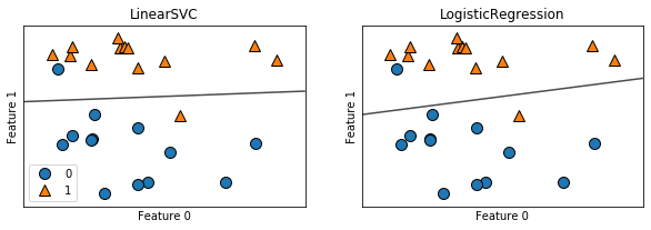
在这张图中， forge 数据集的第一个特征位于 x 轴，第二个特征位于 y 轴，与前面相同。图中分别展示了 LinearSVC 和 LogisticRegression 得到的决策边界，都是直线，将顶部归为类别 1 的区域和底部归为类别 0 的区域分开了。换句话说，对于每个分类器而言，位于黑线上方的新数据点都会被划为类别 1，而在黑线下方的点都会被划为类别 0。

两个模型得到了相似的决策边界。注意，两个模型中都有两个点的分类是错误的。两个模型都默认使用 L2 正则化，就像 Ridge 对回归所做的那样。

对于 LogisticRegression 和 LinearSVC ，决定正则化强度的权衡参数叫作 C 。 C 值越大，对应的正则化越弱。换句话说，如果参数 C 值较大，那么 LogisticRegression 和LinearSVC 将尽可能将训练集拟合到最好，而如果 C 值较小，那么模型更强调使系数向量（w）接近于 0。参数 C 的作用还有另一个有趣之处。较小的 C 值可以让算法尽量适应“大多数”数据点，而较大的 C 值更强调每个数据点都分类正确的重要性。下面是使用 LinearSVC 的图示

mglearn.plots.plot_linear_svc_regularization()

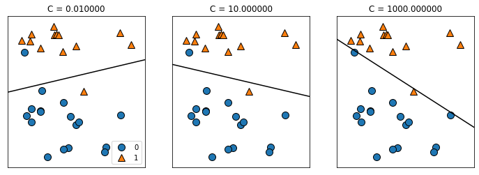
在左侧的图中， C 值很小，对应强正则化。大部分属于类别 0 的点都位于底部，大部分属于类别 1 的点都位于顶部。强正则化的模型会选择一条相对水平的线，有两个点分类错误。在中间的图中， C 值稍大，模型更关注两个分类错误的样本，使决策边界的斜率变大。最后，在右侧的图中，模型的 C 值非常大，使得决策边界的斜率也很大，现在模型对类别 0 中所有点的分类都是正确的。类别 1 中仍有一个点分类错误，这是因为对这个数据集来说，不可能用一条直线将所有点都分类正确。右侧图中的模型尽量使所有点的分类都正确，但可能无法掌握类别的整体分布。换句话说，这个模型很可能过拟合。

与回归的情况类似，用于分类的线性模型在低维空间中看起来可能非常受限，决策边界只能是直线或平面。同样，在高维空间中，用于分类的线性模型变得非常强大，当考虑更多特征时，避免过拟合变得越来越重要。

我们在乳腺癌数据集上详细分析 LogisticRegression ：

from sklearn.datasets import load_breast_cancer
print(help(train_test_split))
cancer=load_breast_cancer()
# stratify  按某个层次分配
X_train,X_test,y_train,y_test=train_test_split(cancer.data,cancer.target,
                                               stratify=cancer.target,random_state=42)
logreg=LogisticRegression().fit(X_train,y_train)
print("Taining set score:{:.3f}".format(logreg.score(X_train,y_train)))
print("Test set score:{:.3f}".format(logreg.score(X_test,y_test)))

Help on function train_test_split in module sklearn.model_selection._split:

train_test_split(*arrays, **options)
    Split arrays or matrices into random train and test subsets
    
    Quick utility that wraps input validation and
    ``next(ShuffleSplit().split(X, y))`` and application to input data
    into a single call for splitting (and optionally subsampling) data in a
    oneliner.
    
    Read more in the :ref:`User Guide <cross_validation>`.
    
    Parameters
    ----------
    *arrays : sequence of indexables with same length / shape[0]
        Allowed inputs are lists, numpy arrays, scipy-sparse
        matrices or pandas dataframes.
    
    test_size : float, int or None, optional (default=None)
        If float, should be between 0.0 and 1.0 and represent the proportion
        of the dataset to include in the test split. If int, represents the
        absolute number of test samples. If None, the value is set to the
        complement of the train size. If ``train_size`` is also None, it will
        be set to 0.25.
    
    train_size : float, int, or None, (default=None)
        If float, should be between 0.0 and 1.0 and represent the
        proportion of the dataset to include in the train split. If
        int, represents the absolute number of train samples. If None,
        the value is automatically set to the complement of the test size.
    
    random_state : int, RandomState instance or None, optional (default=None)
        If int, random_state is the seed used by the random number generator;
        If RandomState instance, random_state is the random number generator;
        If None, the random number generator is the RandomState instance used
        by `np.random`.
    
    shuffle : boolean, optional (default=True)
        Whether or not to shuffle the data before splitting. If shuffle=False
        then stratify must be None.
    
    stratify : array-like or None (default=None)
        If not None, data is split in a stratified fashion, using this as
        the class labels.
    
    Returns
    -------
    splitting : list, length=2 * len(arrays)
        List containing train-test split of inputs.
    
        .. versionadded:: 0.16
            If the input is sparse, the output will be a
            ``scipy.sparse.csr_matrix``. Else, output type is the same as the
            input type.
    
    Examples
    --------
    >>> import numpy as np
    >>> from sklearn.model_selection import train_test_split
    >>> X, y = np.arange(10).reshape((5, 2)), range(5)
    >>> X
    array([[0, 1],
           [2, 3],
           [4, 5],
           [6, 7],
           [8, 9]])
    >>> list(y)
    [0, 1, 2, 3, 4]
    
    >>> X_train, X_test, y_train, y_test = train_test_split(
    ...     X, y, test_size=0.33, random_state=42)
    ...
    >>> X_train
    array([[4, 5],
           [0, 1],
           [6, 7]])
    >>> y_train
    [2, 0, 3]
    >>> X_test
    array([[2, 3],
           [8, 9]])
    >>> y_test
    [1, 4]
    
    >>> train_test_split(y, shuffle=False)
    [[0, 1, 2], [3, 4]]

None
Taining set score:0.955
Test set score:0.958

C=1 的默认值给出了相当好的性能，在训练集和测试集上都达到 95% 的精度。但由于训练集和测试集的性能非常接近，所以模型很可能是欠拟合的。我们尝试增大 C 来拟合一个更灵活的模型：

logreg100 = LogisticRegression(C=100).fit(X_train, y_train)
print("Training set score: {:.3f}".format(logreg100.score(X_train, y_train)))
print("Test set score: {:.3f}".format(logreg100.score(X_test, y_test)))

Training set score: 0.972
Test set score: 0.965

使用 C=100 可以得到更高的训练集精度，也得到了稍高的测试集精度，这也证实了我们的直觉，即更复杂的模型应该性能更好。
我们还可以研究使用正则化更强的模型时会发生什么。设置 C=0.01 ：

logreg001 = LogisticRegression(C=0.01).fit(X_train, y_train)
print("Training set score: {:.3f}".format(logreg001.score(X_train, y_train)))
print("Test set score: {:.3f}".format(logreg001.score(X_test, y_test)))

Training set score: 0.934
Test set score: 0.930

最后，来看一下正则化参数 C 取三个不同的值时模型学到的系数

plt.plot(logreg.coef_.T, 'o', label="C=1")
plt.plot(logreg100.coef_.T, '^', label="C=100")
plt.plot(logreg001.coef_.T, 'v', label="C=0.001")
#指定坐标轴的刻度
plt.xticks(range(cancer.data.shape[1]), cancer.feature_names, rotation=90)
#matplotlib.pyplot.hlines(y, xmin, xmax)表示横线，参数(y的值，横线开始横坐标，横线结束横坐标)
#matplotlib.pyplot.vlines(y, xmin, xmax)表示竖线，参数(x的值，竖线开始纵坐标，竖线结束纵坐标)
plt.hlines(0, 0, cancer.data.shape[1])
# 指定y轴范围
plt.ylim(-5, 5)
plt.xlabel("Coefficient index")
plt.ylabel("Coefficient magnitude")
plt.legend()

Help on function hlines in module matplotlib.pyplot:

hlines(y, xmin, xmax, colors='k', linestyles='solid', label='', *, data=None, **kwargs)
    Plot horizontal lines at each *y* from *xmin* to *xmax*.
    
    Parameters
    ----------
    y : scalar or sequence of scalar
        y-indexes where to plot the lines.
    
    xmin, xmax : scalar or 1D array_like
        Respective beginning and end of each line. If scalars are
        provided, all lines will have same length.
    
    colors : array_like of colors, optional, default: 'k'
    
    linestyles : {'solid', 'dashed', 'dashdot', 'dotted'}, optional
    
    label : string, optional, default: ''
    
    Returns
    -------
    lines : `~matplotlib.collections.LineCollection`
    
    Other Parameters
    ----------------
    **kwargs :  `~matplotlib.collections.LineCollection` properties.
    
    See also
    --------
    vlines : vertical lines
    axhline: horizontal line across the axes
    
    Notes
    -----
    
    
    .. note::
        In addition to the above described arguments, this function can take a
        **data** keyword argument. If such a **data** argument is given, the
        following arguments are replaced by **data[<arg>]**:
    
        * All arguments with the following names: 'colors', 'xmax', 'xmin', 'y'.
    
        Objects passed as **data** must support item access (``data[<arg>]``) and
        membership test (``<arg> in data``).

None

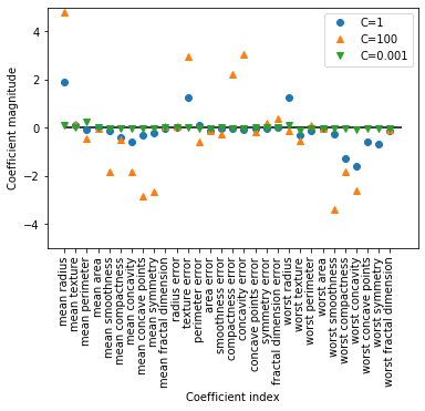
由于 LogisticRegression 默认应用 L2 正则化，所以其结果与图 2-12 中 Ridge 的结果类似。更强的正则化使得系数更趋向于 0，但系数永远不会正好等于 0。进一步观察图像，还可以在第 3 个系数那里发现有趣之处，这个系数是“平均周长”（mean perimeter）。C=100 和 C=1 时，这个系数为负，而C=0.001 时这个系数为正，其绝对值比 C=1 时还要大。在解释这样的模型时，人们可能会认为，系数可以告诉我们某个特征与哪个类别有关。例如，人们可能会认为高“纹理错误”（texture error）特征与“恶性”样本有关。但“平均周长”系数的正负号发生变化，说明较大的“平均周长”可以被当作“良性”的指标或“恶性”的指标，具体取决于我们考虑的是哪个模型。这也说明，对线性模型系数的解释应该始终持保留态度。

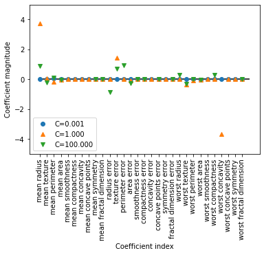
如果想要一个可解释性更强的模型，使用 L1 正则化可能更好，因为它约束模型只使用少
数几个特征。下面是使用 L1 正则化的系数图像和分类精度

for C, marker in zip([0.001, 1, 100], ['o', '^', 'v']):
    lr_l1 = LogisticRegression(C=C, penalty="l1").fit(X_train, y_train)
    print("Training accuracy of l1 logreg with C={:.3f}: {:.2f}".format(
    C, lr_l1.score(X_train, y_train)))
    print("Test accuracy of l1 logreg with C={:.3f}: {:.2f}".format(
    C, lr_l1.score(X_test, y_test)))
    plt.plot(lr_l1.coef_.T, marker, label="C={:.3f}".format(C))
plt.xticks(range(cancer.data.shape[1]), cancer.feature_names, rotation=90)
plt.hlines(0, 0, cancer.data.shape[1])
plt.xlabel("Coefficient index")
plt.ylabel("Coefficient magnitude")
plt.ylim(-5, 5)
plt.legend(loc=3)

Training accuracy of l1 logreg with C=0.001: 0.91
Test accuracy of l1 logreg with C=0.001: 0.92
Training accuracy of l1 logreg with C=1.000: 0.96
Test accuracy of l1 logreg with C=1.000: 0.96
Training accuracy of l1 logreg with C=100.000: 0.99
Test accuracy of l1 logreg with C=100.000: 0.98

6.用于多分类的线性模型

许多线性分类模型只适用于二分类问题，不能轻易推广到多类别问题（除了 Logistic 回归）。将二分类算法推广到多分类算法的一种常见方法是“一对其余”（one-vs.-rest）方法。在“一对其余”方法中，对每个类别都学习一个二分类模型，将这个类别与所有其他类别尽量分开，这样就生成了与类别个数一样多的二分类模型。在测试点上运行所有二类分类器来进行预测。在对应类别上分数最高的分类器“胜出”，将这个类别标签返回作为预测结果。

每个类别都对应一个二类分类器，这样每个类别也都有一个系数（w）向量和一个截距（b）。下面给出的是分类置信方程，其结果中最大值对应的类别即为预测的类别标签：

w[0]∗x[0]+w[1]∗x[1]+…+w[p]∗x[p]+b

多分类 Logistic 回归背后的数学与“一对其余”方法稍有不同，但它也是对每个类别都有一个系数向量和一个截距，也使用了相同的预测方法。

我们将“一对其余”方法应用在一个简单的三分类数据集上。我们用到了一个二维数据集，每个类别的数据都是从一个高斯分布中采样得出的

from sklearn.datasets import make_blobs
X,y=make_blobs(random_state=42)
mglearn.discrete_scatter(X[:,0],X[:,1],y)
plt.xlabel("Feature 0")
plt.ylabel("Feature 1")
plt.legend(["Class 0","Class 1","Class 2"])
print(help(mglearn.discrete_scatter))

Help on function discrete_scatter in module mglearn.plot_helpers:

discrete_scatter(x1, x2, y=None, markers=None, s=10, ax=None, labels=None, padding=0.2, alpha=1, c=None, markeredgewidth=None)
    Adaption of matplotlib.pyplot.scatter to plot classes or clusters.
    
    Parameters
    ----------
    
    x1 : nd-array
        input data, first axis
    
    x2 : nd-array
        input data, second axis
    
    y : nd-array
        input data, discrete labels
    
    cmap : colormap
        Colormap to use.
    
    markers : list of string
        List of markers to use, or None (which defaults to 'o').
    
    s : int or float
        Size of the marker
    
    padding : float
        Fraction of the dataset range to use for padding the axes.
    
    alpha : float
        Alpha value for all points.

None

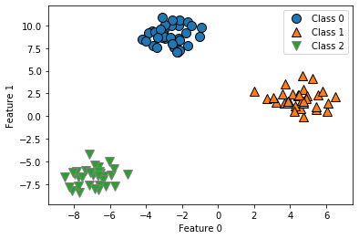
现在，在这个数据集上训练一个 LinearSVC 分类器：

linear_svm=LinearSVC().fit(X,y)
print("Coefficient shape: ", linear_svm.coef_.shape)
print("Intercept shape: ", linear_svm.intercept_.shape)

Coefficient shape:  (3, 2)
Intercept shape:  (3,)

我们看到， coef_ 的形状是 (3, 2) ，说明 coef_ 每行包含三个类别之一的系数向量，每列包含某个特征（这个数据集有 2 个特征）对应的系数值。现在 intercept_ 是一维数组，保存每个类别的截距。

我们将这 3 个二类分类器给出的直线可视化

import numpy as np
mglearn.discrete_scatter(X[:, 0], X[:, 1], y)
line = np.linspace(-15, 15)
for coef, intercept, color in zip(linear_svm.coef_, linear_svm.intercept_, ['b','r','g']):
    plt.plot(line, -(line*coef[0]+intercept)/coef[1], c=color)
plt.ylim(-10,15)
plt.xlim(-10, 8)
plt.xlabel("Feature 0")
plt.ylabel("Feature 1")
plt.legend(['Class 0', 'Class 1', 'Class 2', 'Line class 0', 'Line class 1',
'Line class 2'], loc=(1.01, 0.3))

<matplotlib.legend.Legend at 0x2537d7a06a0>

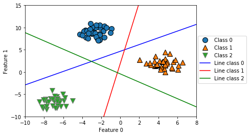
你可以看到，训练集中所有属于类别 0 的点都在与类别 0 对应的直线上方，这说明它们位于这个二类分类器属于“类别 0”的那一侧。属于类别 0 的点位于与类别 2 对应的直线上方，这说明它们被类别 2 的二类分类器划为“其余”。属于类别 0 的点位于与类别 1 对应的直线左侧，这说明类别 1 的二元分类器将它们划为“其余”。因此，这一区域的所有点都会被最终分类器划为类别 0（类别 0 的分类器的分类置信方程的结果大于 0，其他两个类别对应的结果都小于 0）。

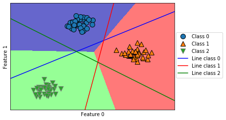
但图像中间的三角形区域属于哪一个类别呢，3 个二类分类器都将这一区域内的点划为“其余”。这里的点应该划归到哪一个类别呢？答案是分类方程结果最大的那个类别，即最接近的那条线对应的类别。下面的例子给出了二维空间中所有区域的预测结果：

mglearn.plots.plot_2d_classification(linear_svm, X, fill=True, alpha=.6)
mglearn.discrete_scatter(X[:, 0], X[:, 1], y)
line = np.linspace(-15, 15)
for coef, intercept, color in zip(linear_svm.coef_, linear_svm.intercept_,
['b', 'r', 'g']):
    plt.plot(line, -(line * coef[0] + intercept) / coef[1], c=color)
plt.legend(['Class 0', 'Class 1', 'Class 2', 'Line class 0', 'Line class 1',
'Line class 2'], loc=(1.01, 0.3))
plt.xlabel("Feature 0")
plt.ylabel("Feature 1")

Text(0, 0.5, 'Feature 1')

7.优点，缺点和参数

线性模型的主要参数是正则化参数，在回归模型中叫作 alpha ，在 LinearSVC 和 Logistic-Regression 中叫作 C 。 alpha 值较大或 C 值较小，说明模型比较简单。特别是对于回归模型而言，调节这些参数非常重要。通常在对数尺度上对 C 和 alpha 进行搜索。你还需要确定的是用 L1 正则化还是 L2 正则化。如果你假定只有几个特征是真正重要的，那么你应该用L1 正则化，否则应默认使用 L2 正则化。如果模型的可解释性很重要的话，使用 L1 也会有帮助。由于 L1 只用到几个特征，所以更容易解释哪些特征对模型是重要的，以及这些特征的作用。

线性模型的训练速度非常快，预测速度也很快。这种模型可以推广到非常大的数据集，对稀疏数据也很有效。如果你的数据包含数十万甚至上百万个样本，你可能需要研究如何使用 LogisticRegression 和 Ridge 模型的 solver=’sag’ 选项，在处理大型数据时，这一选项比默认值要更快。其他选项还有 SGDClassifier 类和 SGDRegressor 类，它们对本节介绍的线性模型实现了可扩展性更强的版本。

线性模型的另一个优点在于，利用我们之间见过的用于回归和分类的公式，理解如何进行预测是相对比较容易的。不幸的是，往往并不完全清楚系数为什么是这样的。如果你的数据集中包含高度相关的特征，这一问题尤为突出。在这种情况下，可能很难对系数做出解释。

如果特征数量大于样本数量，线性模型的表现通常都很好。它也常用于非常大的数据集，只是因为训练其他模型并不可行。但在更低维的空间中，其他模型的泛化性能可能更好。2.3.7 节会介绍几个线性模型不适用的例子。